All about Simple Linear Regression

This article talks about Simple Linear Regression from the scratch – From different types of regression to concepts underlying for evaluation of a model to predicting future values based on regression. The topics covered are –

• Introduction
• Some properties of Simple Linear Regression Model
• Types of Regression
• Estimating the Best Fitting Line
• Properties of Least Squares Line b₀ & b₁
• Statistical Properties of least square estimators (b₀ & b₁)
• Understanding Distributions followed by Sum of Squares of Residuals
• Evaluating Model-Test of Slope Coefficient
• Evaluating Model- ANOVA
• Which test statistic is better?
• Coefficient of Regression
• Confidence Interval of β₁
• Interval Estimation of the mean response
• Prediction Interval for a New Response

 

Introduction

Regression is used to determine relationship between 2 set of variables. The 2 set of variables are dependent and independent variables. Dependent variable may be called as Response variable and independent variable may be referred as predictor, concomitant, controllable, explanatory, covariate variables. Dependent Variable is usually denoted by Ybar and Independent Variable is denoted by Xi, I =1 to p.

Univariate Regression Model is the one which has one dimensional dependent Variable. But if dependent Variable is a vector then we have Multivariate Regression.

Simple Regression is when we have only one independent variable. Multiple Regression is when we have multiple independent variables.

We never know what the true relationship is in between Y and Xs (Dependent and Independent variables respectively) but we assume that there is some function that defines Y in terms of Xs. However, it is very difficult to find out this function. And even if we figure out this function we shall still get different results owing to random errors (measurement limitations, model inadequacies, uncontrollable factors, missing Xs, etc). Thus the model has a deterministic part (the function defining Y in terms of Xs) and Random Noise (Errors).

While regressing Y on Xs we try to approximate the deterministic part(true unknown function f) which can be denoted by β₀+ β₁ X₁+ β₂ X₂+ β₃ X₃+….+β_p-1X_p-1, where βi s are regression coefficients or parameters.  And for random error, we assume that on an average for all the Xs given and a repeated observation of Xs, the Expectation/mean of random noise is 0. This also implies that Deterministic linear model (β₀+ β₁ X₁+ β₂ X₂+ β₃ X₃+….+β_p-1X_p-1) actually represents the locus of means of Y as the set of Xs changes values over repeated observation. Hence, we can say, E (Y|X₁…..X_p-1) = β₀+ β₁ X₁+ β₂ X₂+ β₃ X₃+….+β_p-1X_p-1.

 

Some properties of Simple Linear Regression Model

• E(Y_i), at each value of the predictor, X_i, is a Linear function of the X_i
• The errors, €_i, are Independent.
• The errors, €_i, at each value of the predictor, X_i are normally distributed.
• The errors, €_i, at each value of the predictor, X_i, have Equal variances (denoted σ2).

(Source & Reference: https://onlinecourses.science.psu.edu/stat501/node/253)

 

Types of Regression

• Linear Regression -We call a Regression to be Linear when Regression the βi s parameters are linear.
• First Order Regression – It is the regression where the independent variables used as regressors are not having any further deeper level of association with other variables. (Y = mX+n)
• Higher Order Regression – When the regressors are of higher degrees, let’s say X_i=Z², X_i+1=Z and so on, then first the regression on Y is called Higher (Quadratic when second order and Cubic when third order) Order Regression. (Y = mZ+nZ²+e)

 

Estimating the Best Fitting Line

Scatter Plot – For given (X_i,Y_i), we plot all the (X,Y) for all observations and then try to draw a best fitting line(one which passes through most of the (X,Y) points or which gives least error). There are n number of lines that can pass through these points and in order to determine which is the best fitting line we use Least Squares Estimates method.

Least Squares Estimates Method – Now, that we understand different types of regressions let us consider First Order Linear Regression Y = β₀+β₁X+€  to understand the Least Square Method which determines the best fitting line passing through several points plotted from the observation of (Xi,Yi).

Y = β₀+β₁X+€

The bold underlined part represents the deterministic part/function. Through regression we can approximate some lines Y = b₀+b₁X, where b₀ & b₁ values change for different possible lines. Now, in order to figure out best fitting line, we try to approximate b₀ & b₁ values such that sum of squared differences between the plotted Y (Y_i) values and approximated Y values (b₀+b₁X_i) is minimum for all observations i. That is, we try to minimize the equation below, by taking derivative with respect to b₀ & b₁ and then setting it to 0 to obtain b₀ & b₁. This process is called minimizing the sum of squared prediction errors.

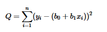
This equation Q is also called as SS_Residuals.

On solving these equations we get the least square estimates of b₀ & b₁ as-

For understanding the calculations in details please refer the following link.

https://www.youtube.com/watch?v=Z_GyV_SuFTI&index=2&list=PLLqEsfz6HOamSu7v9zBZ1IkVcCl2atzWL

b₁ can also be called as Sxy/Sxx.

Interpretation of b1 is simply that when Xi increases by 1 unit Yi increases/decreases by b₁*X_i.

And interpretation of b0 is average Y when Xi is zero.

Thus, Y_pred= b₀+b₁X_i where b₀ & b₁ are obtained from above equations represents “least squares regression line,” or “least squares line” or “estimated regression equation.”

 

Properties of Least Squares Line b₀ & b₁

• Sum of residuals in any regression model that contains an intercept b0 is always 0.
• Sum of observed value equals sum of fitted values
• Sum of Residual value multiplied by weighted regressor value is zero.
• Sum of Residual value weighted by the fitted respondent value is zero.

 

Statistical Properties of least square estimators (b₀ & b₁)

• Both b₀ & b₁ are unbiased estimator of β₀ & β₁
• If the Xi’s are fixed, then b₀ & b₁ is a linear combination of the Yi’s.
• Variance of b₁ is σ²/Sxx
• Variance of b₀ is σ²: {(1/n)+(xbar2/Sxx)}
• Estimation of σ²:
  

For details refer: https://www.youtube.com/watch?v=HcIVc7TI_z0&list=PLLqEsfz6HOamSu7v9zBZ1IkVcCl2atzWL&index=3

 

Understanding Distributions followed by Sum of Squares of Residuals

SS_Res = ∑€_i²

We know that €_I follow Normal distribution with mean 0 and variance σ² which implies that €_I/σ follows N(0,1). And from the property of identically independent distributions the square of iids following normal distribution has chi squared distribution.

Therefore, (€I/ σ²) ~ ϰ₁²

From the least square properties discussed previously, we know that sum of all the €I is zero and Sum of Residual value multiplied by weighted regressor value is zero. Owing to these conditions on €_I there are n-2 degrees of freedom for residuals. That is, there are n-2 errors terms that can be chosen independently but 2 terms have to be chosen in such a way that they follow the 2 conditions mentioned above in this paragraph.

Thus, (SS_residual/ σ²) =∑(€_I/ σ²) ~ ϰ_n-2²

This implies, {(n-2)MS_residual}/ σ² ~ ϰ_n-2² where MS_residual = SS_residual/(n-2). This is useful in testing hypothesis. We will see this in detail while using ANOVA technique to evaluate the models.

 

Evaluating Model-Test of Slope Coefficient

This test is to show if there is a linear relationship between X and Y.

The Null Hypothesis considered here is β₁ = 0 (Indicating No Linear Relationship)

And the alternate hypothesis is β₁ ≠ 0 (Indicating Linear Relationship)

To test this hypothesis, we first find out the distribution followed by b₁ which is an unbiased estimate of β₁ i.e. mean of b₁ is β₁.

As seen earlier the error term follows normal distribution with mean 0 and variance σ2.

And, E (Yi) is β₀+β₁X_i. Thus, Yi follows N (β₀+β₁X_i , σ²).

From this we can say that b1 follows N (β₁, σ²/Sxx) and Z = (b₁– β₁)/ ~ N(0,1)

 

Test Statistic:

Z = (b₁)/ under H₀: β₁ = 0

If σ² is known, we can use Z to test Null hypothesis such that we reject H0 if |Z| > Zα/2.

Usually, we do not know the σ² and hence replace σ² by its estimate MSResidual i.e. SSResidual/(n-2).

t = (b₁– β₁)/(√(MSResidual)⁄(Sxx)) ~ t_n-2

 

Test Statistic:

t = (b₁)/(√(MSResidual)⁄(Sxx)) under H₀: β₁ = 0

We reject H₀: β₁ = 0 if |t| > t _α/2,n-2

 

Evaluating Model- ANOVA

Our model is Y = β₀+β₁X+€ and the fitted line is Y_pred= b₀+b₁X_i  and again the Null hypothesis is  H₀: β₁ = 0. To solve this problem or test this null hypothesis we use Analysis of Variance technique instead of t test mentioned above.

The aim of the ANOVA technique is to find out how much of the total variation of response variable is explained by the regressor variable and how much is left unexplained.

Total unexplained variation in data = ∑(Y_i – Y_pred)2

Let us replace Y_pred by ^Y_i  and Y. denote the average of Y_i for understanding following concepts.

The Variation can be decomposed as follows.

Sum of Squares, naming convention and its meaning is as denoted below.

Following table represents Degrees of Freedom of different sum of squares and provides its justification.

Means Squares are nothing but Sum of Squares divided by Degrees of Freedom which is given in the following table

From all this, we can now create an ANOVA table –

Also, the expected value of MSR is given by

E (MSR) = σ² + b₁² ∑ (Xi – Xbar)²

And that of MSE is given by

E (MSE) = σ²

We have seen earlier that {(n-2)MSresidual}/ σ² ~ ϰ_n-2² and MSReg/ σ² ~ ϰ₁² and under the H0 : β1 = 0, these two entities/distributions are independent.

From the statistical theorem, X~ ϰ_m² and Y~ ϰ_n² such that X and Y are independent then F = (X/m)/(Y/n) ~ F_m,n Distribution.

Thus, F = MSR/MSE follow F_1,n-2 distribution.

 

What does F value denote?

When the F value is 1 it means MSR value is equal to MSE and hence b₁ equals to zero. But if it is large then b₁ is non zero indicating existence of linear relationship between dependent and independent variables.

To test the significance and the hypothesis, we compute F and reject H0:  β₁ = 0 if F > F_α,1,n-2.

 

Which test statistic is better?

While testing simple linear regression, no test is better than the other as F=t². The results obtained are same for whichever test statistic is used for model evaluation. However, while test Multiple Linear Regression, ANOVA approach needs to be used.

 

Coefficient of Regression

It is defined as R² = SSR/ SST. This is one parameter to evaluate the performance of fitted model. To further understand how use this to evaluate model refer following article.

http://thevectormachine.com/index.php/2016/09/19/assessing-linear-regression-model/

 

Confidence Interval of β₁

The aim of confidence interval is to provide a range of b₁ in which the population parameter β₁ would be seen with high probability than giving a point estimate. To achieve this we first find the point estimate and then try to find the sampling distribution of that point estimate b₁.

Least square estimate or point estimate of β₁ is given by Sxy/Sxx.

And we have seen previously that (b₁– β₁)/(√(MSResidual)⁄(Sxx)) ~ t_n-2.

The confidence interval of β₁ is nothing but

P{ -t _α/2,n-2 ≤(b₁– β₁)/(√(MS_Residual)⁄(S_xx)) ≤ t _α/2,n-2 } = 1- α

 

Interval Estimation of the mean response

Again to estimate the mean response interval, we first find point estimation of mean response.

That is for a given x=x_h, expected value of Y is obtained. Let us denote it by E (Y|x=x_h). Then we find out the sampling distribution of this expected value which comes out to be

This when normalized we see that E (Y|x=x_h) follows t_n-2 distribution.

Thus,

100(1-α) % CI on E (Y|x=x_h) is

Where y^_h is the fitted or predicted value.

This CI is minimum at x_i=x_h . It widens as | x_h – x_bar| increases.

 

Prediction Interval for a New Response

Just as we found Confidence Interval Estimation of Mean Response, we find Prediction Interval for a new response.

Where y^_h is the fitted or predicted value.

 

Source & Reference:

https://onlinecourses.science.psu.edu/stat501/node/250

http://www.unc.edu/~nielsen/soci708/m15/m15.htm